3 Methodology
As discussed earlier, tracking datasets provide the position of all players and the ball throughout the match with a temporal resolution of 25fps. This enables us to estimate the players’ covered distance, speed, and acceleration. The potential for extracting information from tracking datasets that is useful for football analytics extends beyond variables related to players’ physical performance. Many tactical metrics has been implemented to decode how the intricate movements of players translate to the football field.
These models provide a scientific perspective for analysing player positioning, decision- making, and team dynamics, illuminating the complex interactions that occur during a match.
Pitch Control is one of the most relevant tactical metrics used to analyse player positioning, decision-making, and team dynamics during a football match. It combines player position and speed with mathematical models that simulate ball and player movement (Spearman 2018).
This thesis proposes to use Pitch Control Models to evaluate how soccer teams interact with the offside line when attacking and defending. Before doing so, we first need to define Pitch Control Models, including their construction and implementation.
3.1 Pitch Control Models
The Pitch Control (PC) at a given location represents the probability of a player or team gaining control of the ball if it moves directly to that location. PC models simulate the dynamics of the ball and the players to evaluate which player would control the ball if it moves to any location on the pitch at any moment. The model captures not only the players’ current position, but also their movement. When players are running at high speeds, they are more likely to control the space they are moving into rather than the space they currently occupy.
To construct this model, we must address the following issues for a given location on the pitch:
- How long it would take for the ball to reach to the position of interest (from its starting position).
- How long would it take for each player to get to that position.
- What is the total probability that each team will control the ball after both the players and the ball have arrived at the desired position?
In the model, the ball is set to move at a constant speed of \(v_b = 54\) \(km/h\), which is approximately the average speed of the ball in the game (Spearman 2018) (See Fig. 3.1)
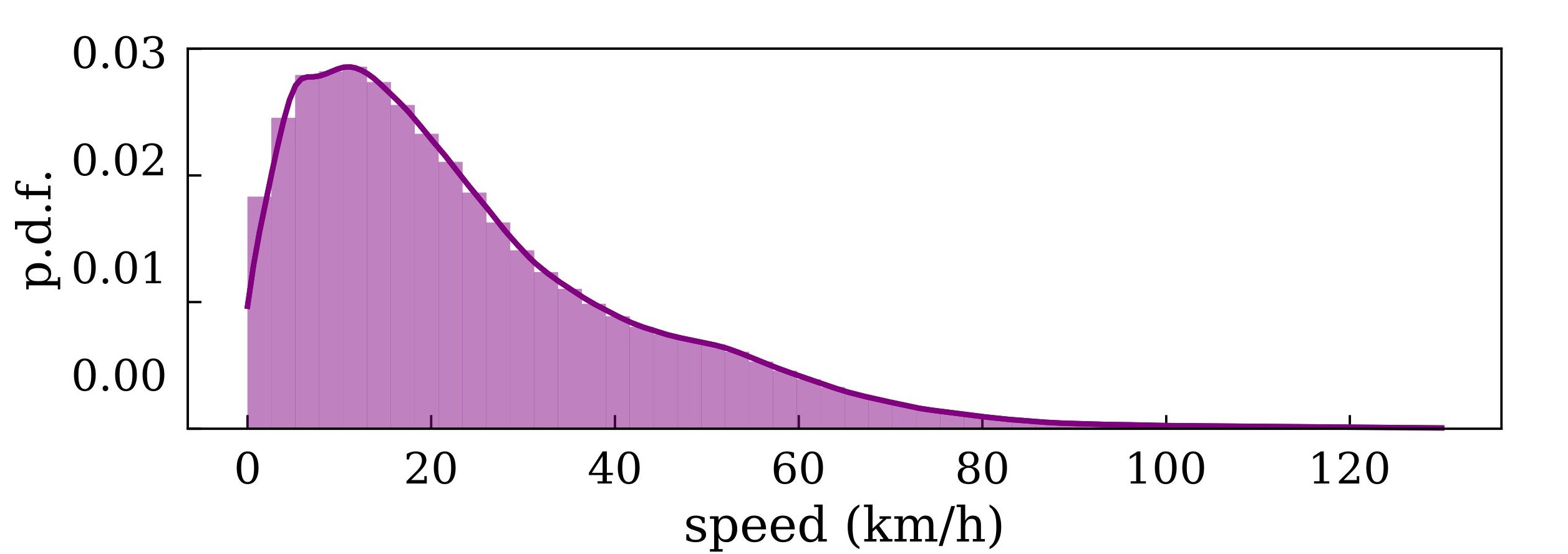
Figure 3.1: p.d.f of the ball speed over a 100 matches from LaLiga 2019-2020 season.
Therefore, the time taken to arrive at the location of interest can be easily calculated as \(t_{b,arr} = \Delta x_b/v_b\), where \(\Delta x_b\) is the distance between the initial and final positions of the ball.
3.1.1 Model assumptions
When considering how long it will take the players to reach the target position, given their initial position and speed, players are assumed to only have a maximum speed of \(v_{max,p} = 18\) \(km/h\), which corresponds to the 95 percentile of the average speed of the players in the game5 (Spearman 2018) (See Fig. 3.2). This upper limit should not be misunderstood as the maximum speed at which players can move, but rather as an estimate of the maximum speed at which they are likely to move when trying to control the ball
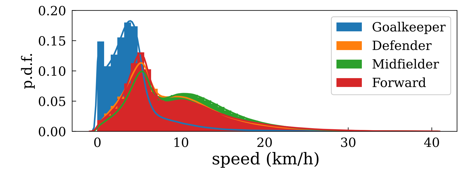
Figure 3.2: p.d.f of the players speed over a 100 matches from LaLiga 2019-2020 season.
To compute the player’s expected arrival time, \(\tau_{exp}(\vec{r};t_r)\) , we use a simple approximation consisting of a two-step process:
- There is an initial reaction time, assumed to be of \(t_{r} = 0.7\) seconds for every player6. This is approximately the time it takes a player moving at maximum speed to come to a complete stop (Spearman 2018). During this reaction time, we assume that players continue to move along their current trajectory without changing speed or direction (reaching a position \(\vec{r}_{\text{react}}\)).
- After this time, we assume that the player runs directly towards the ball at his maximum speed of \(v_{\text{max,p}}\).
\[\begin{align*} \tau_{exp}(\vec{r} ; t_r) = t_r + \frac{|\vec{r} - \vec{r}_{react}|}{v_{max,p}} \end{align*}\]
3.1.2 Control probability
Once we have computed the time it takes for the ball and the players to get to the target location, we need to look at how long it will take each player to control the ball. To do this, we assume that controlling the ball is a stochastic process that follows an exponential distribution with a fixed rate \(\lambda\). The inverse of such a free parameter, \(\lambda^{-1}\), can be thought of as the time it takes a player to gain control of the ball, in seconds. Modeling the process with a exponential distribution, we capture the fact that players who stay closer to the ball for longer are more able to control the ball, (3.1) (Spearman et al. 2017). Thus, for any differential time \(\Delta t\) that a player is near the ball, he has a probability of \(\lambda \cdot \Delta t\) of controlling the ball.
\[\begin{align} F(\Delta t ; \lambda)=1-e^{-\lambda \Delta t} \tag{3.1} \end{align}\]
So far, the model assumes that we know exactly when each player will arrive at the target location. However, we introduce some uncertainty, labelled \(\sigma\), in the arrival time of the players. The reason for including such temporal variability in our model is to account for some effects that have not been explicitly modeled, such as player effort. To model that uncertainty, we will use a Logistic distribution. Thus, the probability of a player intercepting the ball at time T is given by the cumulative distribution function of the sigmoid distribution (Spearman et al. 2017) (See Fig. 3.3).
\[\begin{align*} F_{\text {int }}(\vec{r},T;\sigma, t_r)=\frac{1}{1+e^{-\frac{T- \tau_{exp}(\vec{r} ; t_r)}{\sqrt{3} \sigma / \pi}}} \end{align*}\]
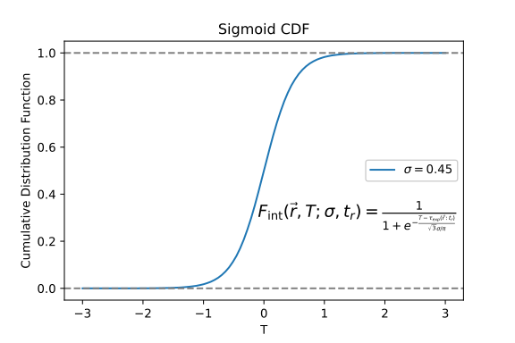
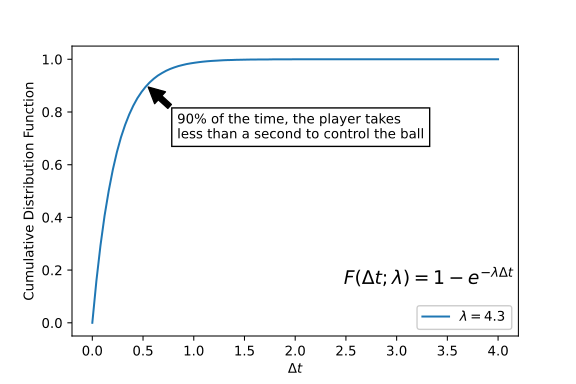
Figure 3.3: The cumulative distribution functions for the two components of the model. a) (left) the time to intercept and b) (right) the time to control the ball. The parameters shown for each are from the global fit described below.
Both \(\lambda\) and \(\sigma\) has been selected according to (Spearman et al. 2017), where they model passes as a Bernoulli trial, with probability mass function
\[\begin{align*} P(k \mid \sigma, \lambda, x)=\left\{\begin{array}{lr} 1-p \text { for } \mathrm{k}=0 \\ p & \text { for } \mathrm{k}=1 \end{array}\right. \end{align*}\]
where \(k \in [0,1]\) is the outcome of the pass. Then, the likelihood of a set of
parameters, \(\sigma\) and \(\lambda\), given outcome \(k\) and the start of the pass \(x\) is:
\[\begin{align*} \mathcal{L}(\sigma, \lambda \mid k, x)=P(k \mid \sigma, \lambda, x) \end{align*}\]
Then, maximizing the product of the likelihood for each pass for a training sample P from tracking and event data from the 2015-2016 Premier League season, the best fit is found at7 \(\sigma=0.45 \pm 0.05 \mathrm{~s} \text { and } \lambda=4.30 \pm 1.14 \mathrm{~s}^{-1}\)
\[\begin{align*} \min _{\sigma, \lambda \in\{\mathbb{R}, \mathbb{R}\}}\left\{-\sum_{i \in P} \log \left[\mathcal{L}\left(\sigma, \lambda \mid k_i, x_i\right)\right]\right\} \end{align*}\]
Using the above components, we recursively construct the partial derivative of the probability that player \(j\) controls a given location \(r\), at time t is
\[\begin{align} \frac{d P P C F_j}{d t}\left(T, \vec{r} , \sigma, \lambda_j, t_r\right)=\left(1-\sum_k P P C F_k\left(t, \vec{r} , \sigma, \lambda_k\right)\right) F_{int,j}(t, \vec{r} , \sigma, t_r) \lambda_j \tag{3.2} \end{align}\]
where \(PPCF_j\) is the Potential Pitch Control Field of player \(j\). \(F_{int,j}(t, \vec{r}, T ; \sigma, t_r)\) is the probability that player \(j\) can reach the target location \(r\) in a given time \(t\), and \(\lambda_j\) is the control rate of such a player 8. Importantly, note that \(\sum_k P P C F_k\left(T, \vec{r} , \sigma, \lambda_k\right)\) accounts for the sum of the Potential Pitch Control Field of the rest of the \(k\) players on the pitch at time \(t\).
By integrating the equation above, Eq. (3.2), \(t \in \left[ t_{ball},t_{ball} + 10 \right]\) seconds, and taking \(P P C F_j\left(t, \vec{r} , \sigma, \lambda_j\right) = 0\) at the beginning of the integration, the probability of control per player is obtained. This probability is then extracted along all the pitch, obtaining a pitch control surface.
Now that we are able to generate the pitch control surface for a frame, we can extend this methodology to measure the quality of each team’s offside strategy. To do this, we will focus on the pitch control generated after the offside line, called Offside Control (OC). To do this, we determine where the offside line is and which players are in an offside position. Then we calculate the pitch control generated by the attacking team after the offside line. If a player is in an offside position, we mark his contribution as ineffective.
The Offside Control was calculated for 100 matches from LaLiga (season 2018 - 2019) using tracking data. We calculated the OC every 2 frames per second of each match. In order to discretise the space efficiently, we decided to reduce our calculations to the half of the pitch of the team not in possession of the ball. We then detect the position of the offside line and calculate the pitch control after it. In this way, we significantly reduce the computation time of the model while maintaining a high spatial resolution (\(50 \times 32\)).
Bibliography
We can impose this assumption for all the players without loss of generality, to simplify the model. Further work to improve the model will be individualize this reaction parameter for each player.↩︎
We can impose this assumption for all the players without loss of generality, to simplify the model. Further work to improve the model will be individualize this reaction parameter for each player.↩︎
See (Spearman et al. 2017) for further details↩︎
We assign the goalkeepers to have a higher control rate, \(\lambda_{GK} = 12.9\) \(s^{-1}\), to ensure that they are likely to claim the ball if it is near them and also to account for the ability of grabbing the ball with their hands↩︎